Contents
- Introduction
- Horn-Schunck Method
- Variational Framework
- Optimization
- Evaluation
- Algorithm Flowchart
- Experimental Results
Introduction
Estimating the motion of every pixel in a sequence of images is a problem with many applications in computer vision, such as image segmentation, object classification, and driver assistance.
In general, optical flow describes a dense vector field, where a displacement vector is assigned to each pixel, which points to where that pixel can be found in another image. An example is shown as below.

This project is a solution for Assignment 3 Optical Flow Estimation of the course Image Processing and Computer Vision (ENGG 5104, CUHK, 2015 Spring). In this project, I implement an algorithm solving the optical flow map (u,v) between two image frames using Horn-Schunck Method.
Horn-Schunck Method
Horn-Schunck method is a classical optical flow estimation algorithm. It assumes smoothness in the flow over the whole image. Thus, it tries to minimize distortions in flow and prefers solutions which show more smoothness. In this assignment, we will implement the modern version of Horn-Schunck method, using pyramid-based coarse-to-fine scheme to achieve better performance, similar to that of Lucas-Kanade method. Many current optical flow algorithms are built upon its framework.
The objective is formulated as a global energy functional which is then minimized. Let the image be p = (x,y) and the underlying flow field be w(p) = (u(p),v(p), 1), where u(p) and v(p) are the horizontal and vertical components of the flow field, respectively. Under the brightness constancy assumption, the pixel value should be consistent along the flow vector, and the flow field should be piecewise smooth. This results in an objective function in the continuous spatial domain

where ∇ is the gradient operator, λ weights the regularization, I1 and I2 are two corresponding images.
Variational Framework
To solve Eq. (1), we use an iterative flow framework. It assumes that an estimate of the flow field is w, and one needs to estimate the best increment dw(dw=(du,dv)), to update w. The objective function in Eq. (1) is then changed to

Let

With first-order Taylor expansion:

In the above equation we add variable p into du and dv to index du and dv in images.
For easy computation, we vectorize u, v, du, dv into U, V, dU, dV, and Dx, Dy to denote derivative filters in x and y direction. The continuous function E(du,dv)in Eq. (2) can be discretized as E(dU,dV).
Optimization
The main idea to solve the above equation is to find dU,dV so that the gradient

We can derive

L is a Laplacian filter defined as

The term of dU in gradient is derived similarly. Therefore, solving the gradient equation can be performed in the following linear system

Evaluation
Having built the pyramids and solve Eq. (8) in each level iteratively, the result in the finest level is obtained. We evaluate optical flow results by two measures: Average Angle Error (AAE) and End Point Error (EPE). They are defined by comparing flow result with the ground truth flow. The lower the AAE and EPE are, the better the optical flow performance is. Also we can visually estimate your result from visualization of the flow map (using flowToColor function).
Algorithm Flowchart
Input: frame1,frame2,λ
Build image pyramid;
Initialize flow = 0;
For i= numPyramidLevel:1
    Initialize flow from previous level;
    Build gradient matrix and Laplacian matrix;
    For j=1:maxWarpingNum
        Warp image using flow vector;
        Compute image gradient Ix, Iy, and Iz;
        Build linear system to solve HS flow;
        Solve linear system to compute the flow;
        Use median filter to smooth the flow map;
    EndFor
EndFor
Output: flow
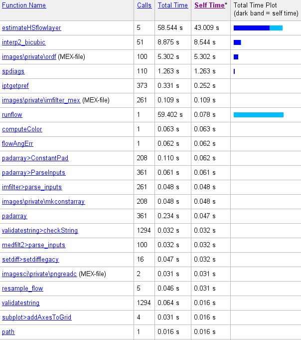
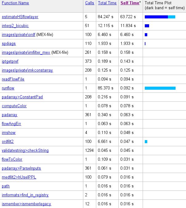
Experimental Results
Five pairs of images are tested, the results as execution time are shown below:


Evaluation measure of picture above: AAE 9.669 average EPE 1.010.


 Evaluation measure of picture above: AAE 9.812 average EPE 0.297.


Some regions in the image groups with visible changes are circled to show that the Warped Image is more similar to frame 1 than frame 2, which indicates that the estimated optical flow is considerately accurate, since the the Warped Image representing frame2 warped to frame1 accroding to the estimated optical flow.